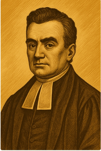
Thomas Bayes (c. 1702–1761): English minister and mathematician whose posthumous "Essay Towards Solving a Problem in the Doctrine of Chances" (1763) introduced what became Bayes' theorem, revolutionizing probabilistic reasoning and modern statistical inference!
Population Proportion Estimation — Frequentist & Bayesian
Enter raw binary data (0/1) or summary (successes k in trials n). Compare frequentist intervals (Wald, Wilson, Clopper–Pearson, Agresti–Coull) with a Beta-posterior credible interval.
Bayesian prior on p (Beta)
Default is Jeffreys Beta(0.5, 0.5). Uniform is Beta(1,1). Or set informative a,b.
Try examples:
Fill inputs and click Compute.
Assumptions & when to worry
- Independent Bernoulli trials; binomial model.
- Wald unreliable for small n or p near 0/1—prefer Wilson or Bayesian.
- Jeffreys prior (Beta(0.5,0.5)) is objective and boundary-friendly.