Probability Tutorial for Biology 231
Basic notation
Applying basic probability to Mendelian genetics
Conditional probability
Probability in statistical analysis
The binomial distribution
Bayes' theorem
The aim of this tutorial is to guide you through the basics of probability. An understanding of probability is the key to success in Mendelian and evolutionary genetics. Along the way, you will be challenged with eight problems to test your understanding of the concepts.
Basic Notation.
- p(A) = the probability of outcome A.
The value of any probability must lie within the range of 0.0 and 1.0. If p(A) = 0.0, then outcome A is impossible. If p(A) = 1.0, then outcome x is guaranteed.
Consider a typical 6-sided die (the singular of dice). Assume that the die is "fair" (i.e., it is equally likely to land with any of its six sides facing up). Define A as 3. What is p(A)? It is simply the probability of rolling a 3: p(A) = 1/6.
- p(~A) = the probability of anything except outcome A.
By definition, p(~A) = 1 - p(A).
Using the above example, what is p(~A)? It is the probability of rolling anything other than a 3. This can be calculated as one minus p(A): 1 - 1/6 = 5/6.
- p(A,B) = the probability of outcome A or outcome B (or both). This is often referred to as joint probability.
If outcomes A and B are mutually exclusive, then p(A,B) = p(A) + p(B). Put another way, the joint probability of outcomes A and B equals the sum of their individual probabilities. This concept is central to the SUM RULE.
Here are a couple examples using the same die. First, define A as the set {1,2}. Define B as the set {4,5,6}. In this example, p(A) = 2/6 (or 1/3); p(B) = 3/6 (or 1/2). Because outcomes A and B are mutually exclusive, p(A,B) = 2/6 + 3/6 = 5/6.
Now let's redefine B as the set {1,3,5}. What is the joint probability of A and B? It is no longer the sum of the individual probabilities, because A and B are not mutually exclusive; they both have the outcome 1 in common. In this example, p(A,B) = p(1,2,3,5) = 4/6.
- p(AB) = the probability of simultaneous outcomes A and B.
If outcomes A and B are independent, then p(AB) = p(A) × p(B). This concept is central to the PRODUCT RULE.
For this example, we will roll a die and flip a quarter. Define A as the set {3,4} and define B as "heads." What is p(AB), the probability that the die lands on either 3 or 4 and simultaneously the quarter lands on heads? If the two processes are independent (i.e., rolling the die has no influence on flipping the coin or vice versa), then we can use the Product Rule: p(AB) = p(A) × p(B) = 2/6 × 1/2 = 1/6.
Applying Basic Probability to Mendelian Genetics.
- Mendel's First Law (Equal Segregation of Alleles). If an organism has the genotype Dd, Mendel's First Law tells us that half of its gametes should bear the D allele and half should bear the d allele. In terms of formal probability, p(D) = 0.5 and p(d) = 0.5. If an individual has the DD genotype, then p(D) = 1.0 and p(d) = 0.0. If an individual has the dd genotype, then p(D) = 0.0 and p(d) = 1.0.
How is this applicable to Mendelian genetics? Consider the following cross: Dd (parent #1) × dd (parent #2). Using formal probability, what is the chance that a particular offspring has the Dd genotype? We know there are only two ways that this can happen: either (i) parent #1 passes on a D allele and parent #2 passes on a d allele (outcome A), or (ii) parent #1 passes on a d allele and parent #2 passes on a D allele (outcome B). Here is what we want to know:
p(A,B).
Since A and B are mutually exclusive outcomes, we can use the Sum Rule and simply add together p(A) and p(B). But we first have to calculate these.
Let's begin with p(A), the probability that the Dd individual passes on a D allele and the dd individual passes on a d allele. It should be apparent that we can use the Product Rule here, since the two parents are passing on alleles independently of each other. The probability that the Dd parent passes on a D allele is 0.5, and the probability that the dd parent passes on the d allele is 1.0. Therefore, p(A) = 0.5 × 1.0 = 0.5.
Now let's move on to p(B), the probability that the Dd parent passes on the d allele and the dd parent passes on the D allele. Again, we can use the Product Rule. The probability that the Dd parent passes on the d allele is 0.5, and the probability that the dd parent passes on the D allele is 0.0 (right?). Therefore, p(B) = 0.5 × 0.0 = 0.0.
So, to finish the problem, we use the Sum Rule. Remember, we want to solve for p(A,B). We've already accepted that the conditions for using the Sum Rule have been met, so p(A,B) = p(A) + p(B) = 0.5 + 0.0 = 0.5.
Was this easier than using a Punnett square? Probably not. However, all of this reasoning is implicit to a Punnett square! A Punnett square is just a visual shortcut for doing the same arithmetic.
- Mendel's Second Law (Independent Assortment of Alleles of Different Genes). It is when we start considering inheritance of two or more genes that using formal probability makes life considerably easier! Consider the following cross: AABbDdEE × aaBbDdEe. Let's start with an easy question: what is the chance that a particular offspring will have the AabbddEE genotype, assuming that all of the genes are independently assorting? Well, we could set up a Punnett square:
| . |
ABDE |
ABdE |
AbDE |
AbdE |
| aBDE |
AaBBDDEE |
AaBBDdEE |
AaBbDDEE |
AaBbDdEE |
| aBDe |
AaBBDDEe |
AaBBDdEe |
AaBbDDEe |
AaBbDdEe |
| aBdE |
AaBBDdEE |
AaBBddEE |
AaBbDdEE |
AaBbddEE |
| aBde |
AaBBDdEe |
AaBBddEe |
AaBbDdEe |
AaBbddEe |
| abDE |
AaBbDDEE |
AaBbDdEE |
AabbDDEE |
AabbDdEE |
| abDe |
AaBbDDEe |
AaBbDdEe |
AabbDDEe |
AabbDdEe |
| abdE |
AaBbDdEE |
AaBbddEE |
AabbDdEE |
AabbddEE |
| abde |
AaBbDdEe |
AaBbddEe |
AabbDdEe |
AabbddEe |
Right. There are 32 boxes (we got off easy... there could have been 64 for 4 genes). Let's find the ones with AabbddEE.
| . |
ABDE |
ABdE |
AbDE |
AbdE |
| aBDE |
AaBBDDEE |
AaBBDdEE |
AaBbDDEE |
AaBbDdEE |
| aBDe |
AaBBDDEe |
AaBBDdEe |
AaBbDDEe |
AaBbDdEe |
| aBdE |
AaBBDdEE |
AaBBddEE |
AaBbDdEE |
AaBbddEE |
| aBde |
AaBBDdEe |
AaBBddEe |
AaBbDdEe |
AaBbddEe |
| abDE |
AaBbDDEE |
AaBbDdEE |
AabbDDEE |
AabbDdEE |
| abDe |
AaBbDDEe |
AaBbDdEe |
AabbDDEe |
AabbDdEe |
| abdE |
AaBbDdEE |
AaBbddEE |
AabbDdEE |
AabbddEE |
| abde |
AaBbDdEe |
AaBbddEe |
AabbDdEe |
AabbddEe |
It looks like there's a 1/32 chance of getting this genotype. Now let's do it the easy way. Define outcome A as Aa, outcome B as bb, outcome D as dd and outcome E as EE. We are interesting in determining p(ABDE), the probability of simultaneously seeing all four outcomes. Because the genes are independently assorting, we can use the Product Rule: p(ABDE) = p(A) × p(B) × p(D) × p(E).
- p(A): the probability of getting Aa from a AA × aa cross is 1.0.
- p(B): the probability of getting bb from a Bb × Bb cross is 0.25.
- p(D): the probability of getting dd from a Dd × Dd cross is 0.25.
- p(E): the probability of getting EE from a EE × Ee cross is 0.5.
Therefore, the probability that the offspring has the AabbddEE genotype is 1.0 × 0.25 × 0.25 × 0.5 = 0.03125 = 1/32.
TEST YOUR UNDERSTANDING.
Let's cross AaBBCcDdEEffGGHh × AaBbccDDEeFfGgHh. Again, we'll assume that the genes are independently assorting.
First, what is the chance that a particular offspring has the AaBbccDDEeFfGghh genotype? If you choose to set up a Punnett square, beware! You'll have 16 columns and 64 rows, for a grand total of 1024 boxes. Don't make any mistakes...
Solution
From the same cross... what is the probability that the offspring has the dominant phenotype for all eight genes, assuming that upper-case alleles are dominant to lower case alleles?
Solution
Conditional Probability
- p(A|B) = the probability of outcome A given condition B. This is not the same as a joint probability or a simultaneous probability.
It turns out that p(A|B) is very easy to calculate: p(A|B) = p(AB) ÷ p(B). Remember, p(AB) is the simultaneous probability of outcomes A and B. The conditional probability of A given B is their simultaneous probability divided by the probability of B.
Here is an example. Define A as 3. Define B as "odd numbers." First, determine p(A), the probability that a fair die lands on 3. The answer is 1/6 .
Now, determine p(A|B), the probability of rolling 3 given that the die lands on an odd number. The answer is 1/3. Why did the answer change? It didn't. We are asking two different questions. In the first case, we wanted to know the overall probability of outcome A. In the second case, We were only interested in the chance of rolling 3 if condition B was satisfied. If the die had landed on 2, 4 or 6, then condition B would not have been satisfied.
Does the arithmetic described above work? The probability of outcome B (rolling an odd number) is 1/2. The simultaneous probability of A and B is the probability of rolling 3, which is 1/6 since this is the only outcome that satisfies both A and B. Using the formula p(A|B) = p(AB) ÷ p(B), our answer is 1/6 ÷ 1/2 = 1/3.
A slightly trickier problem: determine p(A|~B). We are now seeking the probability of rolling 3 given that the die does not land on an odd number. The answer, of course, is zero. Does the math work? The probability of not rolling an odd number is 1/2. However, the probability of simultaneously satisfying A and ~B (i.e., rolling 3 and not rolling an odd number) is zero. So p(A|~B) = 0 ÷ 1/2 = 0.
TEST YOUR UNDERSTANDING.
Let's apply this to a common Mendelian genetics problem. There is a gene in cats that affects development of the spine. Individuals with the MM genotype are phenotypically normal. Individuals with the Mm genotype are tailless (Manx) cats. The mm genotype is developmentally lethal, so zygotes with this genotype do not develop into kittens. If you cross two Manx cats, what fraction of the kittens are expected to be Manx?
Solution
Let's try a different problem. In fruit flies, brown eyes result from a homozygous recessive genotype (br/br). A pair of heterozygous parents produce a son with wild type eye color. He is mated with a brown-eyed female. What is the probability that their first offspring has brown eyes?
Solution
Probability in Statistical Analysis.
For many statistical tests, we are interested in the so-called p-value. This is the probability of obtaining a particular value of a test statistic (or greater) just by chance. In general, we are using the statistical test to contrast observed results (our data) to expected results (those predicted by the hypothesis being tested). [We usually must make certain assumptions about the data in order to use the p-value to reject or fail to reject the hypothesis.] If the difference between the observed and expected results is sufficiently great -- by convention, such that the p-value corresponding to the test statistic value is less than 0.05 -- we reject the hypothesis used to generated the expected results. If the p-value is greater than 0.05, we fail to reject the hypothesis.
How do we put this in terms of formal probability? Define A as "the observed results or any results less likely given the hypothesis" and B as "the hypothesis is correct." If all of the assumptions of the statistical test are valid, then the p-value = p(A|B): the probability of observing the results or any less likely results given that the hypothesis is correct.
Another way to define a p-value is as follows: it is the probability that, if we choose to reject the hypothesis, we are making a mistake! Obviously, we don't like to make mistakes. So we feel better about rejecting a hypothesis if our statistical test gives us a very low p-value.
The Binomial Distribution
A particularly broad class of repeated experiments falls into the category of Bernoulli Trials. By definition, Bernoulli trials have three characteristics:
- the result of each experiment (i.e., trial) is either success or failure (yes or no, true or false, etc.);
- the probability of success is the same for every trial; and
- the trials are independent, such that the results of any particular trial have no effect on any other trials.
If one knows in advance the probability of success (p), then one can predict the exact probability of k successes in N Bernoulli trials. This probability can be written formally as:
p(k|pN) = [N! ÷ (k! × (N-k)!)] × pk × (1-p)N-k.
In terms of formal probability, the probability of k successes given N trials and given probability of success = p. [Note the awkward use of p for two different purposes in the equation.] This formula is the basis of the Binomial Distribution.
Perhaps a more proper way to think about the Binomial Distribution is to consider the distribution, itself. The Binomial Distribution describes the probabilities of all possible outcomes of N Bernoulli trials given probability of success = p. It should be evident that one could observe, in principle, any integer number of successes ranging from 0 to N.
To better understand the Binomial Distribution, it makes sense to break down the formula.
- [N! ÷ (k! × (N-k)!)]. If we perform N trials and don't care which of those trials represent the k successes, we must calculate the number of different ways that we can get k successes. Consider a die-rolling experiment, where we define success as rolling a 3. If we roll the die 4 times, how many different ways are there to get 0, 1, 2, 3 or 4 successes? The following table summarizes this.
| . |
Trial 1 |
Trial 2 |
Trial 3 |
Trial 4 |
| k=0 |
Fail |
Fail |
Fail |
Fail |
| k=1 |
Success |
Fail |
Fail |
Fail |
| Fail |
Success |
Fail |
Fail |
| Fail |
Fail |
Success |
Fail |
| Fail |
Fail |
Fail |
Success |
| k=2 |
Success |
Success |
Fail |
Fail |
| Success |
Fail |
Success |
Fail |
| Success |
Fail |
Fail |
Success |
| Fail |
Success |
Success |
Fail |
| Fail |
Success |
Fail |
Success |
| Fail |
Fail |
Success |
Success |
| k=3 |
Fail |
Success |
Success |
Success |
| Success |
Fail |
Success |
Success |
| Success |
Success |
Fail |
Success |
| Success |
Success |
Success |
Fail |
| k=4 |
Success |
Success |
Success |
Success |
By comparison, the formula gives the following answers:
| k |
N! |
k! |
N-k! |
[N! ÷ (k! × (N-k)!)] |
| 0 |
1 × 2 × 3 × 4 = 24 |
1 (by definition) |
1 × 2 × 3 × 4 = 24 |
24 ÷ (1 × 24) = 1 |
| 1 |
1 × 2 × 3 × 4 = 24 |
1 |
1 × 2 × 3 = 6 |
24 ÷ (1 × 6) = 4 |
| 2 |
1 × 2 × 3 × 4 = 24 |
1 × 2 = 2 |
1 × 2 = 2 |
24 ÷ (2 × 2) = 6 |
| 3 |
1 × 2 × 3 × 4 = 24 |
1 × 2 × 3= 6 |
1 |
24 ÷ (6 × 1) = 4 |
| 4 |
1 × 2 × 3 × 4 = 24 |
1 × 2 × 3 × 4 = 24 |
1 (by definition) |
24 ÷ (24 × 1) = 1 |
- pk × (1-p)N-k. This part of the formula gives the exact probability of k successes and N-k failures for any particular order of successes and failures. The probability of exactly k independent successes, according to the Product Rule, is pk. The probability of exactly N-k independent failures is (1-p)N-k. Again, using the Product Rule, the simultaneous probability of k successes and N-k failures is the product of their individual probabilities. Hence, we get the right side of the binomial formula.
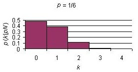
For the die-rolling experiment, the probability of success, p, is 1/6; the probability of failure, 1-p, is 5/6. The following table shows the probabilities of k of N successes for p=1/6:
| k |
pk |
(1-p)(N-k) |
pk × (1-p)(N-k) |
| 0 |
(1/6)0 = 1.0000 |
(5/6)4 = 0.4823 |
1.0000 × 0.4823 = 0.4823 |
| 1 |
(1/6)1 = 0.1667 |
(5/6)3 = 0.5787 |
0.1667 × 0.5787 = 0.0965 |
| 2 |
(1/6)2 = 0.0278 |
(5/6)3 = 0.6944 |
0.0278 × 0.6944 = 0.0193 |
| 3 |
(1/6)3 = 0.0046 |
(5/6)1 = 0.8333 |
0.0046 × 0.8333 = 0.0039 |
| 3 |
(1/6)4 = 0.0008 |
(5/6)0 = 1.0000 |
0.0008 × 1.000 = 0.0008 |
- With the values in these two tables, we can calculate the probability of k successes in N trials if we don't care which trials were successes.
| k |
N! ÷ (k! × (N-k)!) |
× |
pk × (1-p)(N-k) |
= |
p(k|pN) |
| 0 |
1 |
× |
0.4823 |
= |
0.4823 |
| 1 |
4 |
× |
0.0965 |
= |
0.3858 |
| 2 |
6 |
× |
0.0193 |
= |
0.1157 |
| 3 |
4 |
× |
0.0039 |
= |
0.0154 |
| 4 |
1 |
× |
0.0008 |
= |
0.0008 |
Below are binomial distribution plots for 10 Bernoulli trials with three different probabilities of success.
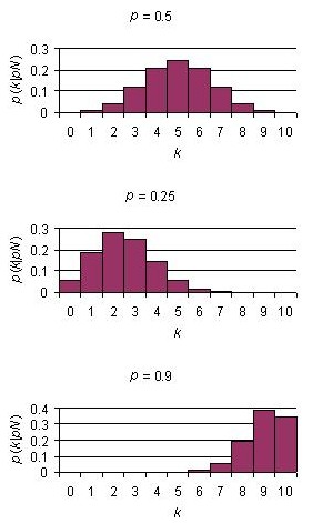
As the number of trials is increased, the binomial distribution becomes smoother. In fact, the normal distribution can be derived mathematically from a binomial distribution with N = infinity and p = 0.5.

TEST YOUR UNDERSTANDING.
Do we really expect the expected results of a cross? Hmmm... In mice, individuals with either the BB or Bb genotype have black fur, while those with the bb genotype have brown fur. [We are ignoring other genes that can interact with this gene to produce other fur colors.] You cross true-breeding black and brown mice to produce heterozygotes, then cross these to produce an F2 generation with sixteen mouse pups. What is the exact probability that you will observe the expected result: twelve black mice and four brown mice?
Solution
Consider, then, the two closest outcomes: eleven black/five brown mice and thirteen black/three brown mice. How much more likely is the expected result than each of these alternative results?
Solution
Bayes' Theorem.
In traditional statistical analysis, we are estimating the probability of observed data given the hypothesis. Sometimes, however, we are interested in the inverse: the probability of a hypothesis given the observed data.
Consider the following scenario. A female human (Gladys) with an autosomal recessive phenotype has mated with a male human (Mickey) with the dominant phenotype. They have three offspring, all of whom show the dominant phenotype. What is the probability that Mickey was a heterozygote?
If we define A as the observed results (i.e., the data) and B as the hypothesis that Mickey is heterozygous and Gladys is homozygous recessive, we are interested in the value of p(B|A). As a conditional probability,
p(B|A) = p(BA) ÷ p(A).
Consider, also, that
p(A|B) = p(AB) ÷ p(B).
It should be obvious that
p(AB) = p(BA).
Therefore, rearranging the formula for p(A|B) and substituting p(BA) for p(AB), we get
p(BA) = p(A|B) × p(B).
If we substitute this into the first formula, we get
p(B|A) = [p(A|B) × p(B)] ÷ p(A).
This equation represents Bayes' Theorem. It has three components:
- p(B) is the prior probability of B. In other words, it is the probability of B before we have any additional information.
- p(A|B) is the probability of A given B.
- p(B|A) is the probability of B given A.
If B is a hypothesis and A is data, then p(B|A) is the posterior probability of B. In other words, it is the probability of B after we have additional information (i.e., A).
At first glance, solving the Mickey/Gladys problem might seem straightforward. We want to calculate the posterior probability of Mickey being a heterozygote given the observation that three children have the dominant phenotype. However, it turns out that only one of the terms on the right side of the formula can actually be calculated with the information provided:
- p(A|B) is the probability of three dominant offspring from a cross of heterozygous and homozygous recessive parents. If we use G and g to represent the alleles of the relevant gene, the cross would be Gg × gg. This cross produces Gg and gg offspring with equal probability (0.5). Since each offspring is produced independently, we use the Product Rule. here is a 0.5 × 0.5 × 0.5 (1/8) chance of having three phenotypically dominant offspring.
The other two terms, p(A) and p(B) can not be calculated with the information provided. We need one more piece of information: the prior probability that Mickey is heterozygous. That is, before we had any offspring data, what was the chance that Mickey was heterozygous? It depends on his parents. If they were both heterozygous, then there is a 2/3 chance that Mickey is heterozygous and a 1/3 chance that he is homozygous dominant. [Remember, we are conditioning these probabilities on the observation that Mickey has the dominant phenotype. Therefore, we only consider the outcomes of the cross that produce dominant offspring.] But if Mickey's parents had different genotypes, the chance that he is a heterozygote will change. So we need more information. Here it is: let's assume that we had prior information that led us to believe that both of Mickey's parents were heterozygous.
Now we can plug in a value for p(B), the prior probability that Mickey is heterozygous and Gladys is homozygous. We know that Gladys has the gg genotype. We also know that Mickey has the dominant phenotype, so his genotype must be either GG or Gg. If both of his parents were heterozygous, then there is a 2/3 change that Mickey is heterozygous. Therefore, we will assume that the prior probability of Mickey being heterozygous and Gladys being homozygous, p(B), is 2/3.
What about p(A)? This actually still has to be calculated. In terms of formal probability,
p(A) = p(A|B) × p(B) + p(A|~B) × p(~B).
So, first, what is p(A|B)? We calculated this already! So, next, what is p(A|~B). That is, what is the probability of seeing three phenotypically dominant offspring if Mickey is not heterozygous? Since Mickey has the dominant phenotype, this means he must have the homozygous dominant genotype. Therefore, there is a 1.0 probability that the three offspring are phenotypically dominant. [GG × gg can only produce Gg offspring.] Therefore, using the formula above, p(A) = 1/8 × 2/3 + 1.0 × 1/3 = 1/12 + 4/12 = 5/12.
We are now ready to calculate the probability that Mickey is a heterozygote given the fact that he and Gladys have three phenotypically dominant offspring. From Bayes' Theorem, p(B|A) = [p(A|B) × p(B)] ÷ p(A) = 1/8 × 2/3 ÷ 5/12 = 1/8 × 2/3 × 12/5 = 0.2.
This is a very important point: if we had made different assumptions about the genotypes of Mickey's parents, we would have obtained a different answer.
This is another very important point: the posterior probability of a hypothesis is generally different than the prior probability of a hypothesis. This is because the posterior probability of a hypothesis is calculated after additional information (the data) has been provided.
Let's take the Mickey/Gladys problem one step farther. Given the data, what are the relative likelihoods of our two competing hypotheses: B, the hypothesis that Mickey is heterozygous and ~B, the probability that Mickey is homozygous(i.e., an individual with the dominant phenotype but not the Gg genotype)? We have already calculated the posterior probability that Mickey is heterozygous (assuming a prior probability of 2/3). We now must calculate the posterior probability that Mickey is homozygous (assuming the same prior probability). This can be written as
p(~B|A) = [p(A|~B) × p(~B)] ÷ p(A).
- p(~B) = 1/3. That is, it is 1 - p(B).
- p(A) = 5/12. This doesn't change!
- p(A|~B) = 1. This was calculated earlier. It is the chance of getting three dominant offspring if Mickey has the GG genotype.
- Therefore, p(~B|A) = [1 × 1/3] ÷ 5/12 = 1/3 × 12/5 = 12/15 = 0.8.
This should actually make sense. If we already calculated that the posterior probability of Mickey being a heterozygote is 0.2, then the posterior probability that he is not a heterozygote should be 1 - 0.2, or 0.8.
So, given the data, what are the relative likelihoods of the two competing hypotheses?
p(B|A) / p(~B|A) = 0.2 / 0.8 = 1/4.
In other words, it is four times more likely that Mickey is a homozygote than it is that he is a heterozygote.
TEST YOUR UNDERSTANDING.
Consider a scenario where healthy individuals heterozygous for a recessive genetic disease represent 18% of the general population, while those with the disease represent 1% of the general population. A healthy male has undergone testing for the recessive allele and learns that he is heterozygous. His spouse is also healthy, but we do not know her genotype. They have a healthy child. What is the posterior probability that she is homozygous?
Solution
This next problem is pretty challenging. How many healthy children must they have before she can be more than 95% confident that she is homozygous? [Note: if they have even one child with the disease, the question is moot. We would know that she is heterozgous.]
Solution